Motion models

Once every epoch sits in a common frame, each star has a time series of positions, and the question becomes what curve to put through it. A motion model is that curve. On this branch these are first-class pluggable classes in flystar.motion_model, all deriving from MotionModel, and FlyStar chooses between them per star rather than imposing one on the whole table.

This is the part of the API that differs most from main.

The models

Every model predicts a position at time \(t\) from parameters it fits and parameters you fix. n_params is how many epochs a star needs before the model is fittable, per coordinate; it is derived as int((n_fit_params + 1) / 2), not set by hand, and it is also the quantity models are ranked by when FlyStar decides what a star can support.

Throughout, \(\Delta t \equiv t - t_0\).

Model	n_params	Fit parameters	Position model
Empty	0	–	\(x(t) =\) fill_value (NaN by default), \(\sigma_x(t) = \infty\). For stars with no usable detection at all.
Fixed	1	\(x_0,\ y_0\)	\(x(t) = x_0\), the weighted mean position – no time dependence. For stars seen once, or held still on purpose.
Linear	2	\(x_0, v_x,\ y_0, v_y\)	\(x(t) = x_0 + v_x\,\Delta t\). Constant proper motion; the workhorse.
Acceleration	3	\(x_0, v_{x0}, a_x,\ y_0, v_{y0}, a_y\)	\(x(t) = x_0 + v_{x0}\,\Delta t + \tfrac{1}{2} a_x\,\Delta t^2\). For stars whose motion visibly curves.
Parallax	3	\(x_0, v_x, \pi,\ y_0, v_y\)	\(x(t) = x_0 + v_x\,\Delta t + \pi\,P_x(t)\). Linear motion plus annual parallax.

Note where \(\pi\) sits in the parallax model: it multiplies the parallax vector \(\boldsymbol{P}(t)\), not \(\Delta t\). Written out for both coordinates,

\[\begin{split}x(t) &= x_0 + v_x\,(t - t_0) + \pi\,P_x(t) \\ y(t) &= y_0 + v_y\,(t - t_0) + \pi\,P_y(t)\end{split}\]

\(\boldsymbol{P}(t)\) is computed by calc_parallax_vector() from the star’s ra/dec, the position angle pa, and the observatory location obsLocation. Note that fit_motion_models currently applies a single obsLocation to every star in the table.

Fixed parameters

Fit parameters are solved for; fixed parameters you supply, either as a column on the table or through fixed_params_dict (scalars apply to every star, arrays must have length N_stars).

Model	Required	Optional
Empty, Fixed	–	–
Linear, Acceleration	\(t_0\)	–
Parallax	\(t_0\), ra, dec	pa (default 0), obsLocation (default 'earth')

\(t_0\) is the one you can always omit. Left unset, it is computed per star as the uncertainty-weighted mean of that star’s own epochs,

\[t_0 = \frac{\sum_i t_i / \sqrt{\sigma_{x,i}^2 + \sigma_{y,i}^2}} {\sum_i 1 / \sqrt{\sigma_{x,i}^2 + \sigma_{y,i}^2}}\]

which puts the reference epoch near the star’s best-measured time and so minimises the covariance between \(x_0\) and \(v_x\).

Fitted parameters land in per-star columns named after the parameter, with uncertainties in <param>_err – vx and vx_err, pi and pi_err. How those errors are computed is below.

Where fixed parameters live

A fixed parameter can come from three places, and both fit_motion_models() and get_predicted_positions() resolve them in the same order:

1. fixed_params_dict, if the key is there

2. a table column of that name

3. table metadata of that name

For a required parameter, exhausting all three raises KeyError. An optional one falls back to the model’s default (pa=0, obsLocation='earth').

The order is worth committing to memory, because the column beats the metadata, and fixed_params_dict beats both. Passing fixed_params_dict to get_predicted_positions therefore overrides whatever the table is carrying, rather than being ignored in its favour.

Fitting writes them back, so a table carries the parameters it was fitted with and get_predicted_positions propagates each star with exactly what its fit used – no need to supply them a second time. The single rule is that the values the fit used end up under <param>, the name the lookup above searches:

Situation	Result
no column of that name, value uniform across stars	table.meta['<param>'], one scalar
no column of that name, value varies per star	a column <param>
a column exists and already agrees	left untouched
a column exists and disagrees	<param> takes the used values; the ones you supplied move to <param>_orig
no column, but metadata of that name disagrees	table.meta['<param>'] is overwritten, and the old value is not kept

Metadata is used only where no column of that name exists, which is what makes it safe: a column would shadow it in the resolution order, so a value written to metadata underneath one could never be read back. Where that is not a risk, one entry in metadata beats the same number repeated down a column of every row.

Note the asymmetry in the last two rows. A conflicting column is preserved under <param>_orig; a conflicting metadata entry is simply overwritten. Metadata is a record of what the table was fitted with, and keeping it in step with the fit is what lets get_predicted_positions propagate without being handed the parameters again – but it does mean that if you need the value the table carried before the fit, you have to keep it yourself.

A column can disagree with the fit because fixed_params_dict outranks it – pass fixed_params_dict={'ra': ...} for a table that already has an ra column and the fit uses the dict. Your column is not overwritten so much as moved aside: <param>_orig keeps it, the same convention MosaicSelfRef follows when it replaces x/y/m with transformed values and leaves x_orig/y_orig/m_orig behind. <param>_orig is written only the first time, so refitting with different values cannot overwrite your original with the previous fit’s substitute.

How a model gets chosen

Two columns govern this, and the asymmetry between them matters:

motion_model_input

Optional, supplied by you. A per-star request.

motion_model_used

Always written by the fit. What actually happened.

fit_motion_models() resolves them so:

1. No motion_model_input column. Each star gets the most complex model in your motion_models list it has enough epochs to support (n_fit >= n_params). If two candidates share the same n_params this is ambiguous and raises AssertionError rather than guessing – supply motion_model_input to disambiguate.

2. With a motion_model_input column. Your request wins wherever the star can support it. A star that cannot falls back to the most complex model it can support, drawn from the union of motion_models and the models named in the column.

Empty and Fixed are always added to the candidate list even if you did not ask for them, so stars detected zero or one time still get a well-defined model instead of failing.

# Everything linear where possible; a few known parallax targets get more.
table['motion_model_input'] = 'Linear'
table['motion_model_input'][is_target] = 'Parallax'

table.fit_motion_models(motion_models=['Linear', 'Parallax'],
                        fixed_params_dict={'ra': ra_deg, 'dec': dec_deg})

# Always check what you got, not what you asked for.
import numpy as np
print(np.unique(table['motion_model_used'], return_counts=True))

Whether such a fallback happens is set by each model’s demote attribute. Most models use 'always'. Orbit uses 'on-missing-init': a star whose orb_* columns already hold a complete set of finite initial elements stays Orbit even with too few epochs (the fit is skipped and the initial elements are kept), while a star without them – for example one newly added to the reference – falls back to a simpler model.

A star demoted to a simpler model has any leftover parameters from its previously-assigned model reset, so vx is never left holding a stale value from an earlier, more complex fit.

Choosing a model versus propagating with one

determine_motion_models() answers a related but distinct question, and the motion_models argument separates them:

• Pass your list to ask which of the models I requested was this star fit with – the answer must stay inside the set you asked for.

• Pass None to ask how well can this star be propagated at all – a property of the star’s own parameters, not of what you chose to fit. A reference star imported with a full parallax solution should be propagated with it even if this run only fit linear motion.

The time-argument contract

Every model’s get_predicted_positions(), and get_predicted_positions(), take times under one rule: shape decides meaning. Nothing is inferred from len(t) happening to equal N_stars.

t	Meaning
scalar	One time, every star.
(N_times,)	One shared grid, every star – always, even when N_times == N_stars.
(1, N_times)	The same, written explicitly.
(N_stars, N_times)	Each star has its own times.

For one time per star, pass a column vector t[:, np.newaxis] of shape (N_stars, 1). A bare 1D array of length N_stars means a shared grid, not per-star times. Any other shape raises ValueError rather than being guessed at. See broadcast_times().

Propagating the whole table to a single new epoch does not need the column-vector form – pass the scalar epoch and let each star’s own \(t_0\) supply the difference:

x, y, xe, ye = table.get_predicted_positions(2026.5)

Uncertainties

Every model reports parameter errors the same way, and it is the way scipy.optimize.curve_fit() does. There is no per-model convention to learn.

Weighting

weighting decides how a per-epoch uncertainty becomes a fit weight, via sigma_from_error() and then weight_from_sigma(), which computes \(w = 1/\sigma^2\):

weighting	\(\sigma_i\) used	Resulting weight
'var' (default)	\(|\sigma_{x,i}|\)	\(w_i = 1/\sigma_{x,i}^2\) – true inverse-variance weighting.
'std'	\(\sqrt{|\sigma_{x,i}|}\)	\(w_i = 1/|\sigma_{x,i}|\) – standard-error weighting, a gentler down-weighting of poorly measured epochs.

Use 'var' unless you have a specific reason: it is the correct choice when your input errors are trustworthy, and it minimises the propagated uncertainty.

The absolute_sigma convention

Let \(\hat{\sigma}_p\) be the formal error on parameter \(p\) from the weighted least-squares covariance, \(\chi^2\) the weighted sum of squared residuals, and \(\nu\) the degrees of freedom (\(n_\mathrm{valid} - n_\mathrm{params}\)). Then:

\[\begin{split}\sigma_p = \begin{cases} \hat{\sigma}_p, & \texttt{absolute\_sigma=True (default)} \\[4pt] \hat{\sigma}_p \sqrt{\chi^2 / \nu}, & \texttt{absolute\_sigma=False} \end{cases}\end{split}\]

True takes your input errors at face value and propagates them. False rescales by the reduced \(\chi^2\), so only the relative magnitudes of the input errors matter and the result reflects the epochs’ own disagreement – the more honest choice when the input errors are known to be systematically underestimated. When \(\nu \le 0\) there is nothing to rescale by and the error is reported as \(\infty\) rather than as a 0/0 NaN.

This is exactly curve_fit’s meaning of the flag, and the equivalence is enforced rather than asserted. flystar/tests/test_motion_model.py fits Fixed, Linear and Acceleration against their own curve_fit call, and Parallax against a joint five-parameter curve_fit over the stacked \([x, y]\) data, comparing parameters, parameter errors and \(\chi^2\) across both weighting schemes, both absolute_sigma settings, several epoch counts including \(\nu = 0\), and nan-padded epochs. Those tests caught a real bug: Fixed had computed \(\chi^2\) as \(\mathrm{resid}^2/\sigma_x^2\) rather than with the fit’s own weights, which coincide only for weighting='var'.

The same flag, with the same meaning, applies to combine_lists(), which collapses a per-list column into a per-star one (x → x0, x0_err). There the reported value is always the uncertainty of the mean, never the scatter of the points. Sigma clipping runs first, so one bad epoch does not drag the average.

Unusable uncertainties get weight zero, not a bad weight

A naive \(1/\sigma^2\) turns a missing or pathological uncertainty into an infinite or NaN weight, corrupting the whole sum rather than excluding one point. weight_from_sigma() instead assigns exactly zero whenever \(\sigma\) is NaN, infinite, exactly zero, or so small that squaring it underflows – and to any epoch marked invalid. Such an epoch drops cleanly out of both the fit and the \(\chi^2\).

If every epoch of a star has weight zero there is no weighted mean to report, and FlyStar does not invent one: the value falls back to the unweighted mean where one is defined, and the uncertainty is \(\infty\). Per-star error columns are filled with inf, not nan, precisely so that “we don’t know” stays distinguishable from “no data” and can never be mistaken for precision.

A degenerate fit is reported, not guessed

When the normal equations are singular – every valid epoch at the same time, say – only some combination of the parameters is constrained, not any individual one. FlyStar detects this against a scaled determinant tolerance and returns fill_value with \(\infty\) errors, rather than the arbitrary minimum-norm answer a pseudo-inverse would hand back.

Empirical errors by bootstrap

The formulae above are analytic and assume the model is right. To get errors that make no such assumption, resample:

table.fit_motion_models(motion_models=['Linear'], bootstrap=100, seed=42)

Each star’s epochs are drawn with replacement bootstrap times, the model is refit on each draw, and the spread of the resulting parameters becomes the reported error.

At the alignment level, calc_bootstrap_errors() does the analogous thing one level up: it resamples the reference stars, re-derives the transformations, and takes the scatter of the transformed positions as the transformation error – capturing uncertainty in the frame itself, which the per-star fit cannot see.

Fitting: one star or a whole table

fit() handles both, dispatching on dimensionality:

• 1D arrays of shape (n_epochs,) – a single star, already filtered to its real epochs.

• 2D arrays of shape (n_stars, n_epochs) – a batch packed rectangularly, with nan marking padding where a star has fewer real epochs than the widest row.

Every model’s solve is closed-form and vectorized across the batch, so both paths run through the same non-iterative code – the single-star case is just a batch of one row. There is no scipy.optimize.curve_fit call and no use_scipy switch on this branch; both were removed in favour of the closed-form solves, which are tested for agreement with curve_fit. In practice you rarely call fit directly: fit_motion_models() is the entry point and takes the 2D path.

Two asymmetries between the two paths

Worth knowing before you call fit directly, because neither is obvious:

The batch path does not fill in \(t_0\). The single-star (1D) path computes the weighted-mean \(t_0\) for you and remembers it on self.fixed_params_dict, so a later get_predicted_positions(t, params) call works with no further arguments. The batch (2D) path does neither – pass fixed_params_dict={'t0': ...} to fit, and the same t0 again to get_predicted_positions:

t2d = np.broadcast_to(t, x.shape)                  # fit dispatches on t.ndim
t0 = np.average(t2d, weights=1./np.hypot(xe, ye), axis=1)
params, param_errs, chi2_x, chi2_y = mm.fit(t2d, x, y, xe, ye,
                                            fixed_params_dict={'t0': t0})[:4]
x_model, y_model, xe_model, ye_model = mm.get_predicted_positions(t_new, params, param_errs,
                                                         {'t0': t0})

Note also that dispatch is on t.ndim, not on x – a 1D t with 2D x takes the single-star path and then fails an assertion about x.

The two paths return different numbers of values. The single-star path returns (params, param_errs), or (params, param_errs, chi2_x, chi2_y, diagnostics) with return_chi2=True. The batch path returns (params, param_errs, chi2_x, chi2_y, diagnostics) regardless of return_chi2. diagnostics is a dict, empty except for Orbit; slice [:4] if you do not need it.

Bootstrap and parallelism

bootstrap=N resamples each star’s epochs N times for empirical parameter errors. It is the one path not vectorized across stars, so it is also the only reason to reach for multiprocessing:

table.fit_motion_models(motion_models=['Linear'],
                        bootstrap=100, seed=42,
                        processes=8)

processes > 1 only spins up a pool once the number of stars needing the per-star path exceeds mp_star_threshold (default 100,000); below that, pool startup and pickling the shared arrays cost more than they save, so fitting stays serial. Measured break-even was between 20,000 and 100,000 stars on a 10-core machine.

Performance

Every motion model in FlyStar is linear in its fit parameters. That is the fact the whole fitting path is built on, and it is not the same as being linear in time: Acceleration is quadratic in \(t\) yet still linear in \((x_0, v_x, a_x)\), because \(t\) only ever appears in the basis \([1, \Delta t, \tfrac{1}{2}\Delta t^2]\) that multiplies them. A model linear in its parameters has a closed-form weighted least-squares solution – the normal equations – so fitting it needs no iterative optimizer, no initial guess, and no convergence check.

Which means the per-star loop was never necessary. The normal equations for 10,000 stars are 10,000 small independent linear systems, and numpy assembles and solves them in a batch:

Model	Params	How the batch is solved
Fixed	1	A weighted average. The whole batch is a pair of .sum(axis=1) calls over the epoch axis.
Linear	2	A 2x2 system per star. The five weighted sums it needs come from .sum(axis=1) across the batch, and the 2x2 is inverted by its closed-form adjugate-over-determinant – rather than building an (n_epochs, n_epochs) diagonal weight matrix and calling an SVD-based pinv per star for what is always a 2x2.
Acceleration	3	The same, one basis function wider: a 3x3 system solved with a batched np.linalg.inv. Hand-deriving a 3x3 adjugate is error-prone for little gain over LAPACK, which is closed-form too.
Parallax	5	Linear once the parallax factors \(P_x, P_y\) are precomputed from each star’s ra/dec. Here \(x\) and \(y\) are not independent – \(\pi\) is shared – so all five parameters are fit jointly from the stacked \([x, y]\) data as one coupled 5x5 system, batched the same way. The \((x_0, v_x)\) and \((y_0, v_y)\) blocks meet only through the shared \(\pi\) row and column.

A non-linear model would not fit this pattern

The batching above is a consequence of linearity in the parameters, not a general technique. Add a model whose parameters enter non-linearly – an orbit, a variable-period term, anything needing a starting guess – and there are no normal equations to assemble: it needs an iterative optimizer, scipy.optimize.curve_fit() or similar, and it will run one star at a time. Such a model can still live alongside these: only the stars actually assigned to it pay the per-star cost, since the model is chosen per star. But do not expect the timings below to carry over to it.

On number of stars

mm_rework is the predecessor branch, which fits star by star through scipy.optimize.curve_fit(); mm_rework_lingfeng is the batched implementation described above. Both were run on the same synthetic data in the same environment at default settings, one after the other rather than concurrently, so that they never competed for cores.

Here the epoch count is held at five – where every model is determined, so nothing below is a fallback – and the number of stars swept from 1,000 to 19,000 in ten steps.

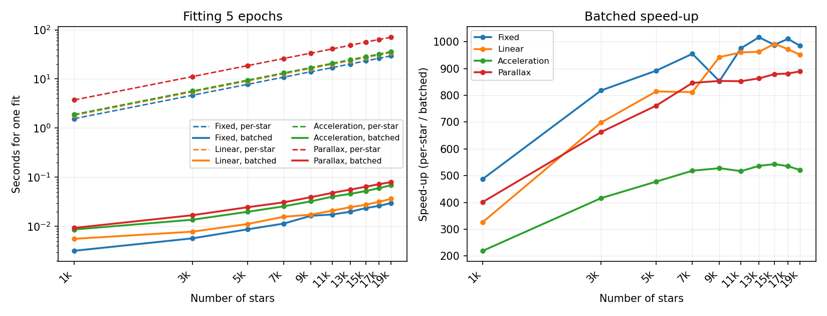
Log-log, unlike the epoch figure below: both branches are strictly linear in the number of stars, and a straight line through the origin is only straight on log-log.

Seconds for one fit at 5 epochs: batched / per-star (speed-up)

Stars	Fixed	Linear	Acceleration	Parallax
1,000	0.003 / 1.6 (488x)	0.006 / 1.8 (327x)	0.009 / 1.9 (219x)	0.009 / 3.7 (402x)
3,000	0.006 / 4.7 (818x)	0.008 / 5.5 (698x)	0.014 / 5.7 (416x)	0.017 / 11.2 (663x)
5,000	0.009 / 7.8 (892x)	0.011 / 9.1 (814x)	0.020 / 9.5 (478x)	0.025 / 18.7 (761x)
7,000	0.011 / 10.9 (955x)	0.016 / 12.8 (812x)	0.026 / 13.3 (518x)	0.031 / 26.1 (846x)
9,000	0.016 / 14.0 (853x)	0.017 / 16.3 (943x)	0.032 / 17.1 (528x)	0.039 / 33.5 (854x)
11,000	0.017 / 17.1 (976x)	0.021 / 20.0 (960x)	0.040 / 20.8 (517x)	0.048 / 41.0 (853x)
13,000	0.020 / 20.2 (1017x)	0.025 / 23.7 (962x)	0.046 / 24.7 (536x)	0.056 / 48.4 (863x)
15,000	0.024 / 23.3 (988x)	0.028 / 27.3 (992x)	0.052 / 28.5 (543x)	0.064 / 56.4 (879x)
17,000	0.026 / 26.4 (1011x)	0.032 / 30.9 (972x)	0.060 / 32.2 (535x)	0.072 / 63.8 (881x)
19,000	0.030 / 29.5 (985x)	0.036 / 34.6 (951x)	0.069 / 36.0 (521x)	0.080 / 70.7 (889x)

The per-star branch is proportional to the star count and nothing else. A straight line fits every one of its four series with \(R^2 = 0.9999\) or better, through an intercept of a few milliseconds at most, at 1.56, 1.82, 1.90 and 3.74 ms per star for Fixed, Linear, Acceleration and Parallax. That is the cost of one Python-level curve_fit call, paid once per star, and it is what makes the model’s complexity visible: fitting five coupled parameters costs a little over twice what fitting one does, per star, every star.

The batched branch is linear too, but with a per-star term 570 to 1,100 times smaller: 1.5, 1.7, 3.3 and 4.0 microseconds per star, on top of a fixed overhead of 1.5 to 4.6 ms that does not depend on the star count at all. The overhead is the vectorized assembly and the batched solve – work done once per table rather than once per star.

So the speed-up grows with the catalogue and then plateaus, from 220-490x at 1,000 stars to 520-990x at 19,000, because at a thousand stars the batched fit’s fixed few milliseconds is still a large fraction of its total and by nineteen thousand it is not. The batched path is at its best exactly where it matters – the large mosaics – and its worst case is a catalogue small enough to fit in the time it takes to read the file.

On number of epochs

The same comparison the other way round: 10,000 stars held fixed, and the epoch count swept. The grid is two epochs, then three to nineteen in steps of two – two is the fewest anything here can fit, and is kept because it is where the more complex models are not yet determined and fall back to a simpler one.

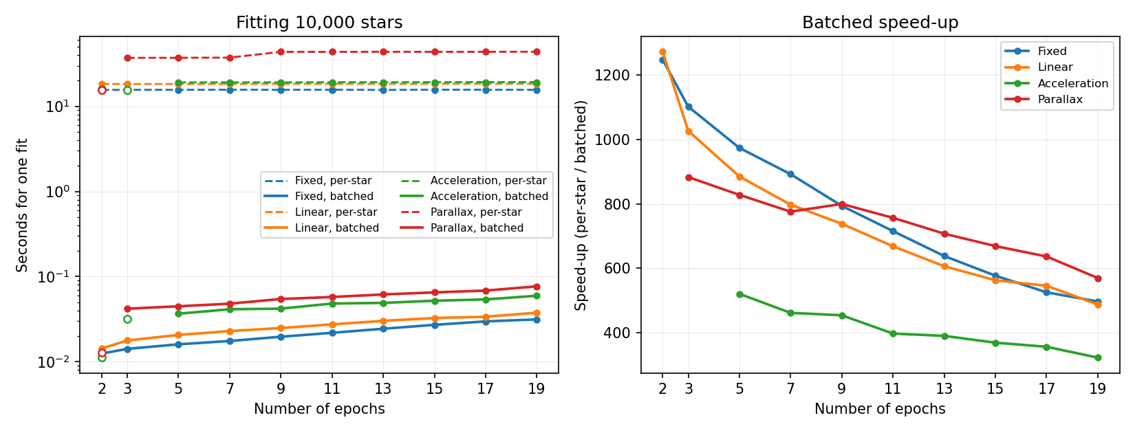
Solid lines are batched, dashed per-star; note the log scale on the left, where the two are three orders of magnitude apart. Hollow markers are cells that did not fit the model of their column at all, so the lines break rather than run through them and the right panel draws no ratio for them – see the footnote.

Seconds for one fit of 10,000 stars: batched / per-star (speed-up)

Epochs	Fixed	Linear	Acceleration	Parallax
2	0.012 / 15.6 (1248x)	0.014 / 18.2 (1272x)	0.011 / 15.7 (not comparable) *	0.013 / 15.6 (not comparable) *
3	0.014 / 15.6 (1102x)	0.018 / 18.2 (1026x)	0.032 / 15.7 (not comparable) *	0.042 / 37.1 (883x)
5	0.016 / 15.6 (973x)	0.021 / 18.3 (885x)	0.037 / 19.1 (520x)	0.045 / 37.1 (828x)
7	0.018 / 15.6 (892x)	0.023 / 18.3 (797x)	0.041 / 19.1 (461x)	0.048 / 37.3 (776x)
9	0.020 / 15.6 (794x)	0.025 / 18.4 (738x)	0.042 / 19.1 (454x)	0.055 / 43.6 (799x)
11	0.022 / 15.7 (715x)	0.027 / 18.4 (668x)	0.048 / 19.2 (397x)	0.058 / 43.6 (756x)
13	0.024 / 15.6 (638x)	0.030 / 18.3 (606x)	0.049 / 19.2 (390x)	0.062 / 43.7 (707x)
15	0.027 / 15.7 (577x)	0.033 / 18.4 (563x)	0.052 / 19.2 (369x)	0.065 / 43.6 (669x)
17	0.030 / 15.6 (525x)	0.034 / 18.4 (545x)	0.054 / 19.2 (356x)	0.069 / 43.6 (636x)
19	0.031 / 15.6 (497x)	0.038 / 18.4 (487x)	0.060 / 19.2 (322x)	0.077 / 43.7 (570x)

* Three cells do not time the model their column names. At two epochs neither Acceleration (3 parameters per direction) nor Parallax (5, fitted jointly) has as many data points as parameters, so both branches fall back, to Fixed on both sides, and those two cells simply repeat the Fixed column. At three epochs Acceleration has exactly as many points per direction as parameters, and here the branches disagree: the batched one fits it, with no degrees of freedom left, so the model passes exactly through the data and there is no residual to estimate an uncertainty from – the parameter errors come back infinite. The predecessor instead requires strictly more epochs than parameters, and demotes those stars past Linear all the way to Fixed, so that cell would be timing Acceleration against Fixed.

Two shapes stand out. The per-star branch is flat in the number of epochs and set almost entirely by the number of stars – 10,000 Python-level optimizer calls cost the same whether each is handed 2 points or 19. The batched branch instead grows mildly with epochs, roughly doubling across the grid, which is the only part of the work that is genuinely proportional to the amount of data. Between them the speed-up falls from about 1250x at two epochs to 320-570x at nineteen – which is not the batched fit degrading, but the flat cost it is measured against staying flat while its own grows. That is the opposite direction to the star sweep above, and the two together say why: more stars scale both branches, so their ratio tends towards the ratio of their per-star costs, while more epochs scale only the batched one.

The batched fit’s cost is also nearly independent of how complicated the model is: a 5x5 coupled Parallax solve lands within a factor of three of a 1x1 Fixed weighted average, because both are one vectorized assembly plus one batched solve, and neither iterates.

Three caveats on reading these numbers. Each cell is a single run on one machine, though a stable one: every per-star series holds to better than 1% across the whole grid, the single exception being Parallax, which steps up once between 7 and 9 epochs and is flat either side of it – in three separate runs, so that step is real. Second, each model is given one throwaway fit on a tiny table before it is timed: the first fit of a model in a process pays a one-time set-up that the rest do not, about 0.03 s for Parallax – roughly two thirds of a whole batched 10,000-star fit – which would otherwise land entirely on whichever cell was timed first. Third, the comparison is of fitting only: bootstrap is excluded throughout, as it is the one path still per-star and so is unaffected by any of this.

The two sweeps overlap at 10,000 stars and 5 epochs, and agree there: the table above gives Fixed as 0.016 / 15.6 s at five epochs, and the star sweep brackets it with 0.016 / 14.0 at 9,000 stars and 0.017 / 17.1 at 11,000.

How it was measured

The script below produced both tables and both figures. Comparing two branches needs two checkouts, so it takes the flystar to time as an argument, and runs once per sweep per branch, then once more per figure to plot. The figures are committed, so building this documentation runs none of it.

"""
Time the motion-model fits on both branches and draw the figures used by the
Performance section of docs/motion_models.rst.

Two sweeps: wall-clock against the number of epochs, at a fixed 10,000 stars,
and against the number of stars, at a fixed 5 epochs.

The comparison spans two branches, so it needs two checkouts of flystar. Add
one as a worktree, time each sweep on each, then plot:

    git worktree add /tmp/wt_mmrework mm_rework

    python docs/benchmark_motion_models.py epochs /tmp/wt_mmrework \\
        mm_rework /tmp/epochs_per_star.json
    python docs/benchmark_motion_models.py epochs . \\
        mm_rework_lingfeng /tmp/epochs_batched.json

    python docs/benchmark_motion_models.py stars /tmp/wt_mmrework \\
        mm_rework /tmp/stars_per_star.json
    python docs/benchmark_motion_models.py stars . \\
        mm_rework_lingfeng /tmp/stars_batched.json

    python docs/benchmark_motion_models.py plot-epochs \\
        /tmp/epochs_batched.json /tmp/epochs_per_star.json
    python docs/benchmark_motion_models.py plot-stars \\
        /tmp/stars_batched.json /tmp/stars_per_star.json

Timing runs are separate processes so that each imports the flystar it is
timing, and are run one after another rather than concurrently so that they do
not compete for cores. The figures are committed, so building the documentation
never runs any of this.
"""
import contextlib
import io
import json
import os
import sys
import time
import warnings

import numpy as np

MODELS = ['Fixed', 'Linear', 'Acceleration', 'Parallax']
FIXED_PARAMS = {'ra': 18.0, 'dec': -30.0, 'pa': 0.0, 'obsLocation': 'earth'}

# The epoch sweep holds the number of stars fixed, and the star sweep holds the
# number of epochs fixed at a value where every model here is determined -- so
# that nothing in that sweep is a fallback.
EPOCHS = [2] + list(range(3, 21, 2))
N_STARS = 10_000
STARS = list(range(1000, 20_000, 2000))
N_EPOCHS = 5


def make_table(n_stars, n_epochs, seed=1):
    """Build a StarTable of linearly moving stars, observed at every epoch."""
    from flystar.startables import StarTable

    rng = np.random.default_rng(seed)
    t = np.tile(np.linspace(2015., 2015. + 2*(n_epochs - 1), n_epochs), (n_stars, 1))
    x0 = rng.uniform(0, 1000, (n_stars, 1))
    y0 = rng.uniform(0, 1000, (n_stars, 1))
    vx = rng.normal(0, 0.3, (n_stars, 1))
    vy = rng.normal(0, 0.3, (n_stars, 1))
    dt = t - t.mean()
    x = x0 + vx*dt + rng.normal(0, 0.05, (n_stars, n_epochs))
    y = y0 + vy*dt + rng.normal(0, 0.05, (n_stars, n_epochs))
    m = np.tile(rng.uniform(12, 19, (n_stars, 1)), (1, n_epochs))
    e = np.full((n_stars, n_epochs), 0.05)

    return StarTable(name=np.array([f'S{i:06d}' for i in range(n_stars)]),
                     x=x, y=y, m=m, xe=e, ye=e, me=e, t=t)


def time_one(branch, model, n_epochs, n_stars=N_STARS):
    """Time a single fit, and report which model the stars actually got."""
    from flystar import motion_model as MM

    tab = make_table(n_stars, n_epochs)

    t0 = time.perf_counter()
    with contextlib.redirect_stdout(io.StringIO()):
        if branch == 'mm_rework_lingfeng':
            tab.fit_motion_models(motion_models=[model],
                                  fixed_params_dict=FIXED_PARAMS, verbose=False)
        else:
            # The old API: one model for everything, and Parallax needs an
            # instance carrying the parameters that are fixed_params_dict now.
            mmd = ({'Parallax': MM.Parallax(RA=FIXED_PARAMS['ra'],
                                            Dec=FIXED_PARAMS['dec'],
                                            PA=FIXED_PARAMS['pa'],
                                            obsLocation=FIXED_PARAMS['obsLocation'])}
                   if model == 'Parallax' else {})
            tab.fit_velocities(default_motion_model=model, motion_model_dict=mmd,
                               show_progress=False, verbose=False)
    elapsed = time.perf_counter() - t0

    # Which model the stars actually got, not just whether it was the one
    # asked for: too few epochs for the requested model and both branches
    # quietly fall back, so a cell can time something other than its label.
    used = np.asarray(tab['motion_model_used']).astype(str)
    names, counts = np.unique(used, return_counts=True)
    return elapsed, float(np.mean(used == model)), str(names[counts.argmax()])


def sweep_points(axis):
    """The (x value, n_stars, n_epochs) of each cell of a sweep."""
    if axis == 'epochs':
        return [(n_epochs, N_STARS, n_epochs) for n_epochs in EPOCHS]
    return [(n_stars, n_stars, N_EPOCHS) for n_stars in STARS]


def run_timings(axis, flystar_dir, branch, out_json):
    warnings.filterwarnings('ignore')
    flystar_dir = os.path.abspath(flystar_dir)
    sys.path.insert(0, flystar_dir)
    import flystar
    assert flystar.__path__[0].startswith(flystar_dir), flystar.__path__

    print(f'{axis} sweep, branch={branch}, flystar={flystar.__path__[0]}', flush=True)
    results = {}
    for model in MODELS:
        # One throwaway fit on a tiny table first. The first fit of a model in
        # a process pays a one-time set-up the rest do not -- ~0.03 s for
        # Parallax, roughly two thirds of a whole batched 10,000-star fit,
        # which would otherwise land entirely on whichever cell was timed
        # first. At the widest epoch grid point, so that the model being warmed
        # up is one the stars actually get: where there are fewer epochs than
        # parameters the fit falls back, warming the wrong path.
        time_one(branch, model, max(EPOCHS), n_stars=50)

        for x, n_stars, n_epochs in sweep_points(axis):
            elapsed, frac, used = time_one(branch, model, n_epochs, n_stars=n_stars)
            results[f'{model}|{x}'] = {'sec': elapsed, 'frac_used': frac,
                                       'used_model': used, 'n_stars': n_stars,
                                       'n_epochs': n_epochs}
            print(f'  {model:13} {n_stars:6d} stars {n_epochs:2d} epochs: '
                  f'{elapsed:8.3f}s ({frac*100:.0f}% got {model}, '
                  f'most got {used})', flush=True)

    json.dump({'branch': branch, 'axis': axis, 'results': results},
              open(out_json, 'w'), indent=1)
    print('wrote', out_json, flush=True)


def plot(axis, batched_json, per_star_json, out_png=None):
    import matplotlib
    matplotlib.use('Agg')
    import matplotlib.pyplot as plt

    if out_png is None:
        name = ('motion_model_performance.png' if axis == 'epochs'
                else 'motion_model_performance_stars.png')
        out_png = os.path.join(os.path.dirname(os.path.abspath(__file__)),
                               '_static', name)
    batched = json.load(open(batched_json))['results']
    per_star = json.load(open(per_star_json))['results']
    xs = np.array([x for x, _, _ in sweep_points(axis)])

    def series(res, model, key='sec'):
        return np.array([res[f'{model}|{x}'][key] for x in xs])

    colors = dict(zip(MODELS, plt.get_cmap('tab10').colors))
    fig, (ax1, ax2) = plt.subplots(1, 2, figsize=(11, 4.2))

    for model in MODELS:
        c = colors[model]
        per, bat = series(per_star, model), series(batched, model)
        # A cell where the requested model was not what the stars actually got
        # timed a fallback instead, so it is not a like-for-like comparison:
        # draw it hollow, break the line rather than run it through a model it
        # did not fit, and quote no ratio between two different models.
        same = ((series(per_star, model, 'frac_used') == 1)
                & (series(batched, model, 'frac_used') == 1))

        ax1.plot(xs, np.where(same, per, np.nan), '--', color=c, lw=1.4,
                 label=f'{model}, per-star')
        ax1.plot(xs, np.where(same, bat, np.nan), '-', color=c, lw=1.8,
                 label=f'{model}, batched')
        for y in (per, bat):
            ax1.plot(xs[same], y[same], 'o', color=c, ms=4)
            ax1.plot(xs[~same], y[~same], 'o', ms=5, mfc='white', mec=c, mew=1.2)
        ax2.plot(xs, np.where(same, per/bat, np.nan), 'o-', color=c, ms=4,
                 lw=1.8, label=model)

    if axis == 'epochs':
        xlabel, held = 'Number of epochs', f'{N_STARS:,} stars'
        ticks, ticklabels = xs, [str(x) for x in xs]
    else:
        xlabel, held = 'Number of stars', f'{N_EPOCHS} epochs'
        ticks, ticklabels = xs, [f'{x//1000}k' for x in xs]

    ax1.set(xlabel=xlabel, ylabel='Seconds for one fit', yscale='log',
            title=f'Fitting {held}')
    if axis == 'stars':
        # Both branches are linear in the number of stars, which is a straight
        # line only on log-log; on a log y against a linear x it reads as a
        # curve, which is the opposite of the point.
        ax1.set_xscale('log')
        ax2.set_xscale('log')
    ax1.legend(fontsize=7.5, ncol=2, loc='center right')
    ax2.set(xlabel=xlabel, ylabel='Speed-up (per-star / batched)',
            title='Batched speed-up')
    ax2.legend(fontsize=8)

    for ax in (ax1, ax2):
        ax.set_xticks(ticks)
        # Rotated on the star axis: ten labels bunch up towards the top of a
        # log scale, and dropping every other one would leave an end unlabelled.
        ax.set_xticklabels(ticklabels, rotation=45 if axis == 'stars' else 0,
                           ha='right' if axis == 'stars' else 'center')
        ax.set_xticks([], minor=True)      # a log axis adds its own otherwise
        ax.grid(alpha=0.25, lw=0.6)

    fig.tight_layout()
    fig.savefig(out_png, dpi=150)
    print('wrote', out_png)


if __name__ == '__main__':
    mode = sys.argv[1]
    if mode in ('epochs', 'stars'):
        run_timings(mode, *sys.argv[2:5])
    else:
        plot(mode.replace('plot-', ''), *sys.argv[2:])

Adding new models

New motion models are welcome, and adding one does not mean touching the fitting machinery. A model is a single class in flystar.motion_model that subclasses MotionModel, declares what it fits and what it needs held fixed, and implements two methods. There is no registry to edit: motion_model_map() discovers models through MotionModel.__subclasses__(), so the class is selectable by name – motion_models=['Wobble'] – as soon as the module defining it is imported.

It has to be a direct subclass

__subclasses__() is not recursive. Subclassing Linear to reuse its parts produces a model that never appears in the map and cannot be selected by name at all. Inherit from MotionModel and call into Linear if you want to borrow from it.

What to declare

Attribute	Meaning
name	The string users pass. Names are resolved with str.capitalize(), so keep it one capitalised word.
fit_param_names	Every fitted parameter, x-direction first, then y, with any parameter shared between the two last – Parallax is ['x0', 'vx', 'y0', 'vy', 'pi'].
n_fit_params	len(fit_param_names).
n_params	Parameters per direction, int((n_fit_params + 1) / 2). It doubles as the fewest distinct epochs the model can be fitted from, and as the sort key that orders models by complexity.
required_fixed_param_names	Names that must be resolvable from fixed_params_dict, a column or metadata, or fitting raises KeyError.
optional_fixed_params	{name: default} for the ones that fall back instead (Parallax’s {'pa': 0., 'obsLocation': 'earth'}).
fixed_param_names	required_fixed_param_names + list(optional_fixed_params).
demote	Optional; defaults to 'always'. What to do with a star that requests this model but has fewer than n_params epochs: 'always' demote, 'never' keep, or 'on-missing-init' keep only if every fit_param_names column already holds a finite initial value. Use the last two only if run_fit returns the initial values when there are too few epochs.

What to implement

Method	Contract
get_predicted_positions	(t, fit_params, fit_param_errs=None, fixed_params_dict=None), returning (x, y) – or (x, y, xe, ye) when errors are passed in. This is what propagation calls, so it must honour the time-argument contract above; use broadcast_times() rather than reimplementing it. Write the model’s functional form directly here, on (N_stars, N_times) arrays.
run_fit	(t, x, y, xe, ye, valid, fixed_params_dict=None, weighting='var', absolute_sigma=True, fill_value=np.nan, verbose=True), returning (params, param_errs, chi2x, chi2y) with shapes (n_stars, n_fit_params), the same, (n_stars,) and (n_stars,). Stars with fewer valid epochs than parameters must come back as fill_value / inf / nan rather than as whatever the arithmetic produced.

The skeleton, then, is:

class Wobble(MotionModel):
    name = 'Wobble'
    fit_param_names = ['x0', 'vx', 'y0', 'vy', 'amp']
    n_fit_params = len(fit_param_names)
    n_params = int((n_fit_params + 1) / 2)

    required_fixed_param_names = ['t0', 'period']
    optional_fixed_params = {'phase': 0.}
    fixed_param_names = required_fixed_param_names + list(optional_fixed_params)

    def get_predicted_positions(self, t, fit_params, fit_param_errs=None, fixed_params_dict=None):
        ...      # dt = broadcast_times(t, ...) - t0, then per direction
                 # x = x0 + vx*dt + amp * np.sin(2*np.pi*dt/period + phase)

    def run_fit(self, t, x, y, xe, ye, valid, fixed_params_dict=None, **kw):
        ...      # whole batch in, (params, param_errs, chi2x, chi2y) out

Pick n_params with the others in mind

Which model each star gets is decided by how many distinct epochs it has, matched against the candidate models’ n_params with numpy.digitize() – which needs those values to be unique across the models being fitted together. They are not unique in the tree already: Acceleration (6 parameters, 3 per direction) and Parallax (5, fitted jointly, also 3) collide, so

table.fit_motion_models(motion_models=['Acceleration', 'Parallax'])

raises AssertionError rather than guessing. The way to fit two models of equal complexity in one pass is a motion_model_input column naming the model per star, which replaces the epoch-count heuristic with your choice and lifts the uniqueness requirement.

Non-linear models

Everything in the tree today is linear in its parameters, which is why the fits are closed-form and batched (see Performance above). A model that is not – an orbit, a free period, anything needing a starting guess – does not fit that pattern, and does not have to.

run_fit is a batch interface, not a promise of a closed form. A model whose fit cannot be vectorized satisfies the same signature by looping inside it:

def run_fit(self, t, x, y, xe, ye, valid, fixed_params_dict=None, **kw):
    n_stars, _ = x.shape
    params = np.full((n_stars, self.n_fit_params), kw.get('fill_value', np.nan))
    param_errs = np.full((n_stars, self.n_fit_params), np.inf)
    chi2x = np.full(n_stars, np.nan)
    chi2y = np.full(n_stars, np.nan)

    for i in range(n_stars):
        good = valid[i]
        if good.sum() < self.n_params:
            continue                       # leave fill_value / inf / nan
        popt, pcov = curve_fit(...)        # one star at a time
        params[i], param_errs[i] = popt, np.sqrt(np.diag(pcov))
        chi2x[i], chi2y[i] = ...

    return params, param_errs, chi2x, chi2y

Two things make that acceptable rather than a regression. The cost is paid only by the stars actually assigned to your model, since the model is chosen per star and each is fitted with its own. And the measurements above put a number on what it costs: a per-star curve_fit loop runs at roughly 1.6 to 3.7 milliseconds per star, against 1.5 to 4.0 microseconds for a batched fit – so a non-linear model over a 10,000-star mosaic should be expected to take tens of seconds, and to dominate the runtime of any table it is used on.

If your model is linear in its parameters but you are unsure whether it can be batched, it can: assemble the normal equations with .sum(axis=1) over the epoch axis and solve them with a batched numpy.linalg.inv(), exactly as Acceleration does.

Testing a new model

flystar/tests/test_motion_model.py has the patterns worth copying:

• Agreement with scipy, star by star – test_scipy_agreement_* fit the same synthetic data with scipy.optimize.curve_fit() and compare parameters, parameter errors and \(\chi^2\). This is the test that catches an algebra slip in a hand-derived solve, and it is worth writing first.

• The time-argument contract – test_model_time_shape_contract checks that each accepted shape of t gives the documented output shape and that anything else raises.

• The fixed-parameter round trip – fit, then get_predicted_positions() with nothing passed, and confirm the model is still selected. This is what fails when a new fixed parameter is written somewhere the lookup does not search.